AI-Matrix
Multidimensional data analyzer.
Project maintained by Recoskie Hosted on GitHub Pages — Theme by mattgraham
Indexed contents
| Introduction: Link |
| The basic algorithm: Link |
| The geometry of higher dimensions: Link |
| Fast dimensional subtraction: Link |
| Decoding dimensional iteration: Link |
| The matrix structure: Link |
| Golden ratio/Quasicrystals: Link |
| Can AI become self aware: Link |
Introduction
I put together a basics document that demonstrates how information and data can be deconstructed into their basic elements, a process that quantum computing can expedite basics link.This algorithm is a faster, accelerated version of reversing information and data to build advanced, accurate data models for AI.
All examples on this page can be modified, so you can change the examples to see the effects.
Solving a dimensional set
Let's start with a one-dimensional set and show how it builds and solves sequentially. Starting from here will help you see how it works.
A one-dimensional set counts by one or by two per number.
So, let's build a one-dimensional set that is 7 more per number.
  var data = [];

  var end = 8;

  var start = 1;

  var per1 = 7;

  for (var i1 = 0; i1 < end; i1++)
  {
    data[i1] = start;

    for (var i2 = 0; i2 < i1; i2++)
    {
      data[i1] += per1;
    }
  }

  console.log(data);
This simple little code creates a set with a starting value of 1. You can change the starting value to anything by changing
var start = 1;
from 1 to any number you wish.The second loop adds 7 more to each value. You can change the added amount to anything you like by changing
var per1 = 7;
from 7 to any number you want, then run the code again.Lastly, the
var end = 8;
can be changed to a bigger number than 8 if you want to make the set longer.The starting amount is always the first digit in the set.
In the case of the example I gave you, we ended up with the following set, starting with one and adding by 7 per value.
1,8,15,22,29,36,43,50
In math, we call these sigma summations. The first number is 1, which solves the problem of the starting amount for our sumitation.
Then, all you have to do is subtract the next number from the previous number.
The next number after 1 is 8, so 8-1=7.
You then move to the next number in the set, moving from 1 to 8. The number after 8 is 15. So 15-8=7.
You do this with all the numbers in the set. This solves the first-dimensional loop or sumitation as it solves the difference between the numbers per iteration.
8-1=7
15-8=7
22-15=7
29-22=7
36-29=7
43-36=7
50-43=7
This gives us how much is added per value. The difference is the same across all numbers, making a set of 7,7,7,7,7,7,7 per value.
Subtracting the set of 7,7,7,7,7,7,7 the same way will give a set of 0,0,0,0,0,0. Which means there is nothing left in the set.
Solving a 2-dimensional set
In the previous example, subtracting the next number from the previous number finds the added value.
I will show you what happens when you add another loop outside our first loop.
  var data = [];

  var end = 8;

  var start = 0;

  var per1 = 1;

  var per2 = 2;

  for( var i1 = 0; i1 < end; i1++ )
  {
    data[i1] = start;

    for( var i2 = 0; i2 < i1; i2++ )
    {
      data[i1] += per1;

      for( var i3 = 0; i3 < i2; i3++ )
      {
        data[i1] += per2;
      }
    }
  }

  console.log(data);
In this example, we create a square using a 2D set, which is the calculation X2, similar to stacking lines of added units on top of each other per value.
In the geometry section, we will talk about what a square is.
Our set is 0,1,4,9,16,25,36,49. So, the first number in the set is 0. Which means the starting value is 0.
var start = 0;
Subtracting the next value into the previous value gives us.1-0=1
4-1=3
9-4=5
16-9=7
25-16=9
36-25=11
49-36=13
This gives us the set 1,3,5,7,9,11,13. The first result will be the first dimension, which is 1.
var per1 = 1;
Subtracting the numbers 1,3,5,7,9,11,13. Going next number by the previous number again.3-1=2
5-3=2
7-5=2
9-7=2
11-9=2
13-11=2
This solves the difference in the second dimension. Which is two more.
var per2 = 2;
Doing the subtraction of 2,2,2,2,2,2 gives us 0,0,0,0,0 things left.After each subtraction of all numbers, the first value is the per-added amount of each loop put inside each other.
It also does not matter if we start analyzing the set from the value 16 as we end up with the starting value of 16 as it still reduces to the following:
var start=16;
withvar per1=9;
andvar per2=2;
This continues the pattern from 16 onward as 16,25,36,49,64,81,100,121. This also applies to the first-dimensional set and higher-dimensional sets. This makes solving dimensional sequences position-independent.The first number without any subtraction will be the starting value.
The first number after the subtraction of all numbers will be per1.
The first number after the subtraction of all numbers again will be per2.
The first number after the subtraction of all numbers again would be per3. Except we end up with 0,0,0,0,0 things left in the third dimension.
You lose one number with each subtraction into all numbers because there is no number to subtract the previous number into at the end of the set.
So, to solve a five-dimensional pattern per iteration (per-added amount) requires at least six numbers in a set, including the starting value.
You can do the math and change per1 and per2 to whatever you like.
The geometry of higher dimensions
I decided to create this section later to show the structure of higher dimensions.
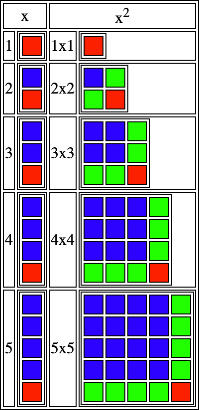 The small number above x is how many times the number is multiplied against itself per value.
The blue squares are the amount that existed before we moved to the next value. The red and green squares are the added units per value.
In the first dimension, we only add one new unit, which can be added together one unit at a time. We input five into our function, and we can add five sevens together if that is the size of the units, or we can just say x is multiplied by 7.
When we multiply the number by itself, we expand this pattern vertically and horizontally.
In the second dimension, we have to add two lines that add by one, shown as green squares that join at one unit.
When we input five into our function, it adds them together as follows:
Green line to corner
1+
1+(1) +
1+(1+1) +
1+(1+1+1) +
1+(1+1+1+1)
Each row is the green line to the corner. The first loop can only add a single unit at the start of each row as a one-dimensional line from blue sqaures to red square, but now we must add another one-dimensional line inside this loop that does the same thing in the () per row as we move down the line shown as the green squares.
We can add the one-dimensional lines in () to make the following whole values.
Green line to corner
1+
1+(1) +
1+(2) +
1+(3) +
1+(4)
We have two green lines that join to the corner as we grow in size in two-dimensional space in which we only have to multiply the added line per unit by 2.
Bottom and right side to corner
1+
1+(1)*2 +
1+(2)*2 +
1+(3)*2 +
1+(4)*2 = 25
Each row now leads to 1x1=1, 2x2=4, 3x3=9, 4x4=16, 5x5=25. The neat part is that we can take away the added unit at the start of each line.
x2-x=0,2,6,12,20 which is 0, 0+2, 0+2+4, 0+2+4+6, 0+2+4+6+8.
1x1-1=0
2x2-2=2
3x3-3=6
This removes the added unit, shown as the red square per square. Dividing it by 2 gives us a set that adds a one-dimensional sequence per value. It was only 2 in size per square because of the two sides.
(x2-x)÷2=0,1,3,6,10, which is 0, 0+1, 0+1+2, 0+1+2+3, 0+1+2+3+4.
As objects fall, they get faster per second. To be exact, 33 feet more per second. We can add this together using two loops or multiply our equation by 33.
((x2-x)÷2)*33=0,33,99,198,330, which is 0,0+33,0+33+66,0+33+66+99,0+33+66+99+132.
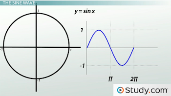
In math, we call these quadratic equations, which means we never have to use two loops inside each other to add such values together. We show the two loops that create the quadratic as two sigma with the second inside the first. Quadratics are good at producing curves and showing an object's path when you throw it as it is pulled toward the earth.
At 2x2, we have two squares stacked on top of each other when we multiply by 2 again, making 2x2x2, and at 3x3x3, we have 3 squares stacked on top of each other. This adds a new square, similar to how we have two lines that make our square using two loops. Adding the third loop, we can add another square per square on top of each other into a cube.
A cube becomes the following continuation pattern in which we add the two-dimensional lines together.
Cube from square expansion
1+
1+(1) +
1+(2) + (1) +
1+(3) + (1+2) +
1+(4) + (1+2+3)
Next, we change the numbers we added per row into whole numbers.
Cube from square expansion
1+
1+(1) +
1+(2) + (1) +
1+(3) + (3) +
1+(4) + (6)
A cube has six sides, so the two-dimensional and three-dimensional lines are multiplied by 6. This could be shown graphically by connecting green lines on six sides, but it is unnecessary as you should understand what is happening.
Cube from square expansion
1+
1+(1)*6 +
1+(2)*6 + (1)*6 +
1+(3)*6 + (3)*6 +
1+(4)*6 + (6)*6 = 125
Each row corsponds to the folowing values 1x1x1 = 1, 2x2x2 = 8, 3x3x3 = 27, 4x4x4 = 64, and 5x5x5 = 125. There is no possible way to add this together using only two loops, as we must add the two-dimensional lines together per row to stack the squares in three-dimensional space.
Multiplying the cube by itself creates a four-dimensional space of cubes per cube and adds another amount to add by on an imaginary axis or line outside the cube. Four dimensions and higher are real, but we only perceive three dimensions visually with our eyes.
Multiplying is much faster than adding our results together with loops nested inside one another per dimension. All forms of counting sequentially by different amounts per dimension can be reduced into simple, fast calculations using multiplication.
Changing the amounts you added per loop inside each other back into equations is explained in the decoding dimensional iteration section.
Higher dimensional sequences and counting of things exist in nature and the world around us.
5-Dimensional set with subtraction
You can solve how much is added per dimension with each subtraction into all numbers, with the first number being the difference.
I will make it so that you can create any five-dimensional set you like in this code. At the end of the code, each number is subtracted from the previous one, and the first value after each subtraction should always be the number of units we added per dimension.
Each per iteration value is set to what x5 is.
  var data = [];

  var end = 8;

  var start = 0;

  var per1 = 1;

  var per2 = 30;

  var per3 = 150;

  var per4 = 240;

  var per5 = 120;

  for( var i1 = 0; i1 < end; i1++ )
  {
    data[i1] = start;

    for( var i2 = 0; i2 < i1; i2++ )
    {
      data[i1] += per1;

      for( var i3 = 0; i3 < i2; i3++ )
      {
        data[i1] += per2;

        for( var i4 = 0; i4 < i3; i4++ )
        {
          data[i1] += per3;

          for( var i5 = 0; i5 < i4; i5++ )
          {
            data[i1] += per4;

            for( var i6 = 0; i6 < i5; i6++ )
            {
              data[i1] += per5;
            }
          }
        }
      }
    }
  }

  console.log("data = "+data);

  var s1 = data[0], s2 = data[1], s3 = data[2], s4 = data[3], s5 = data[4], s6 = data[5], s7 = data[6], s8 = data[7];

  //The starting value.

  console.log("\r\nBegin subtraction\r\n");

  //Subtract next number to previous number.

  s1 = s2 - s1; s2 = s3 - s2; s3 = s4 - s3; s4 = s5 - s4; s5 = s6 - s5; s6 = s7 - s6; s7 = s8 - s7;

  //The first-dimension.

  console.log( [s1,s2,s3,s4,s5,s6,s7] );

  //Subtract next number to previous number.

  s1 = s2 - s1; s2 = s3 - s2; s3 = s4 - s3; s4 = s5 - s4; s5 = s6 - s5; s6 = s7 - s6;

  //The second-dimension.

  console.log( [s1,s2,s3,s4,s5,s6] );

  //Subtract next number to previous number.

  s1 = s2 - s1; s2 = s3 - s2; s3 = s4 - s3; s4 = s5 - s4; s5 = s6 - s5;

  //The third-dimension.

  console.log( [s1,s2,s3,s4,s5] );

  //Subtract next number to previous number.

  s1 = s2 - s1; s2 = s3 - s2; s3 = s4 - s3; s4 = s5 - s4;

  //The fourth-dimension.

  console.log( [s1,s2,s3,s4] );

  //Subtract next number to previous number.

  s1 = s2 - s1; s2 = s3 - s2; s3 = s4 - s3;

  //The fifth-dimension.

  console.log( [s1,s2,s3] );

  //Subtract next number to previous number.

  s1 = s2 - s1; s2 = s3 - s2;

  //The sixth-dimension.

  console.log( [s1,s2] );

  //Subtract next number to previous number.

  s1 = s2 - s1;

  //The zenith-dimension.

  console.log( [s1] );
This code does the subtraction for you. You can change per1 to per5 and even change the start value to whatever you like; even negative or fractional values can be used. The first number after each subtraction is the value that produced the set. We also lose one number each time as there is no number to subtract the last value into. You can change each amount to whatever you like. Or you can do the math yourself.
Faster way of subtracting
Instead of subtracting the next number from the previous with all numbers to find the amount of each dimensional loop, we can calculate them.
The starting amount will always be the first number in the set.
s1 = s1 * 1;We do not need to subtract all the numbers to know the first difference, as it is the second number minus the first number. We only subtracted the rest of the set as the differences need to be reversed in each loop well sumitation.
s1 = s1 * 1;
s2 = s2 - (s1 * 1);
The value s2 matches the first per amount in the second subtraction of all numbers. Previously, in the geometry of higher dimensions, I showed how a square becomes the following sequence 1, 1+1, 1+1+1, 1+1+1+1 per row and how this continues to higher dimensions.
Instead of subtracting all numbers, we can use s1 and s2 to calculate the added amount. Multiplying s2 by 1, 1+1, 1+1+1, 1+1+1+1 per row calculates what s2 is per amount without subtracting the following values from the previous values.
s1 = s1 * 1;
s2 = s2 - (s1 * 1);
s3 = s3 - (s1 * 1 + s2 * 2);
s4 = s4 - (s1 * 1 + s2 * 3);
s5 = s5 - (s1 * 1 + s2 * 4);
s6 = s6 - (s1 * 1 + s2 * 5);
s7 = s7 - (s1 * 1 + s2 * 6);
s8 = s8 - (s1 * 1 + s2 * 7);
The value s3 now matches the third amount in the second subtraction of all numbers.
Multiplying s3 by 1, 1+2, 1+2+3, 1+2+3+4 per row calculates what s3 is per amount outside of s2 (square) by adding the combined one-dimensional lines that made the square.
s1 = s1 * 1;
s2 = s2 - (s1 * 1);
s3 = s3 - (s1 * 1 + s2 * 2);
s4 = s4 - (s1 * 1 + s2 * 3 + s3 * 3);
s5 = s5 - (s1 * 1 + s2 * 4 + s3 * 6);
s6 = s6 - (s1 * 1 + s2 * 5 + s3 * 10);
s7 = s7 - (s1 * 1 + s2 * 6 + s3 * 15);
s8 = s8 - (s1 * 1 + s2 * 7 + s3 * 21);
So then s4 is 1, 1+3, 1+3+6, 1+3+6+10, 1+3+6+10+15, 1+3+6+10+15+21 = 4, 10, 20, 35 which are the added lines of the cubes.
You can view it as taking away the amount added per dimension as we find each per added amount. Additionally, you can produce the same pattern from the 5-dimensional set with the subtraction code example demonstrated earlier on this page by adding up the number of times we subtracted the same values into themselves after each subtraction of all numbers per row.
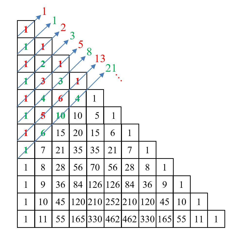
This shortcut removes repeated subtractions. In the following picture is an image of the values we multiplied by.

As you can see in this image, the ones can be added together to form the counting numbers, and the counting numbers can be added together to make triangular numbers. Multiplying the counting numbers by 7 will create a sequence that counts by 7. Multiplying both the counting numbers by 1 and triangular numbers by 2 creates a square.
1x1 + 0x2 = 1
2x1 + 1x2 = 4
3x1 + 3x2 = 9
4x1 + 6x2 = 16
Multiplying the added amounts for the cube, which are 1, 6, and 6, to the counting, triangular and tetrahedral numbers make the cube.
1x1 + 0x6 + 0x6 = 1
2x1 + 1x6 + 0x6 = 8
3x1 + 3x6 + 1x6 = 27
4x1 + 6x6 + 4x6 = 64
You can set each per added amount to whatever you like, and the output will be exactly the amount you set using the dimensional subtraction pattern.
  var data = [];

  var end = 8;

  var start = 7;

  var per1 = 3;

  var per2 = 1;

  var per3 = -9;

  var per4 = 12;

  var per5 = 13;

  for( var i1 = 0; i1 < end; i1++ )
  {
    data[i1] = start;

    for( var i2 = 0; i2 < i1; i2++ )
    {
      data[i1] += per1;

      for( var i3 = 0; i3 < i2; i3++ )
      {
        data[i1] += per2;

        for( var i4 = 0; i4 < i3; i4++ )
        {
          data[i1] += per3;

          for( var i5 = 0; i5 < i4; i5++ )
          {
            data[i1] += per4;

            for( var i6 = 0; i6 < i5; i6++ )
            {
              data[i1] += per5;
            }
          }
        }
      }
    }
  }

  console.log(data);

  var s1 = data[0], s2 = data[1], s3 = data[2], s4 = data[3], s5 = data[4], s6 = data[5], s7 = data[6], s8 = data[7];

  //Each per value per dimensional iteration.

  var o = [];
  o[0] = s1 * 1;
  o[1] = s2 - (o[0] * 1);
  o[2] = s3 - (o[0] * 1 + o[1] * 2);
  o[3] = s4 - (o[0] * 1 + o[1] * 3 + o[2] * 3);
  o[4] = s5 - (o[0] * 1 + o[1] * 4 + o[2] * 6 + o[3] * 4);
  o[5] = s6 - (o[0] * 1 + o[1] * 5 + o[2] * 10 + o[3] * 10 + o[4] * 5);
  o[6] = s7 - (o[0] * 1 + o[1] * 6 + o[2] * 15 + o[3] * 20 + o[4] * 15 + o[5] * 6);
  o[7] = s8 - (o[0] * 1 + o[1] * 7 + o[2] * 21 + o[3] * 35 + o[4] * 35 + o[5] * 21 + o[6] * 7);

  console.log("Decoded per Value = " + o + "");
This makes solving the starting value for each iteration much faster. This gives us the same result as the 5-dimensional set with subtraction without repeated subtractions, which are shrunk into how many times it occurred per row in iteration.
Solving sets to math functions
The per-added amount values up to the fifth dimension are as follows:
| Single Calculation. | start | per1 | per2 | per3 | per4 | per5 | Result. |
| x | 0 | 1 | 0 | 0 | 0 | 0 | 0,1,2,3,4,5,6,7 |
| x2 | 0 | 1 | 2 | 0 | 0 | 0 | 0,1,4,9,16,25,36,49 |
| x3 | 0 | 1 | 6 | 6 | 0 | 0 | 0,1,8,27,64,125,216,343 |
| x4 | 0 | 1 | 14 | 36 | 24 | 0 | 0,1,16,81,256,625,1296,2401 |
| x5 | 0 | 1 | 30 | 150 | 240 | 120 | 0,1,32,243,1024,3125,7776,16807 |
You can create this table by multiplying values and subtracting the set until you have zero left.
The last per-added amount you get is the number of sides the dimensional shape has.
x ends with 1 as it is a straight line with one surface.
x2 ends with 2 as it is a square with two sides/surfaces.
x3 ends with 6 as it is a cube with six sides/surfaces.
x4 ends with 24 as it has 24 sides in the fourth-dimension.
x5 ends with 120 as it has 120 sides in the fifth-dimension.
The number of sides can be calculated by multiplying the number of dimensions by the previous.
1! = 1 is 1
2! = 1x2 is 2
3! = 1x2x3 is 6
4! = 1x2x3x4 is 24
5! = 1x2x3x4x5 is 120
In math, this is called the factorial function, in which 5! is the calculation of 1x2x3x4x5 up to 5, giving us 120.
It is well known that a 4D shape is a tesseract with 24 sides and maybe 4D space time.
I will not discuss the relationship of all higher dimensions to reality as this page is to explain the quantum AI matrix and data analyzer algorithm.
If you persist in learning what the higher dimensions are, then the following video may help 0D to 11D explained advanced.
Mixing calculations
When we add x2+x5 together, we are adding the per-added amounts together.
We end up with the following set of numbers: 0, 2, 36, 252, 1040, 3150, 7812 using the calculation.
When we subtract the values 0, 2, 36, 252, 1040, 3150, 7812 till left with all zero, we find that it breaks down as start = 0, per1 = 2, per2 = 32, per3= 150, per4 = 240, per5 = 120.
The added amounts for x2 is start = 0, per1 = 1, per2 = 2, and the added amounts for x5 is start = 0, per1 = 1, per2 = 30, per3 = 150, per4 = 240, per5 = 120.
If we add the added amounts for both x2+x5 together, 0+0, 1+1, 2+30, 0+150, 0+240, 0+120 we end up with start = 0, per1 = 2, per2 = 32, per3 = 150, per4 = 240, per5 = 120, which is the same as the set of numbers that the calculation reduced back into.
So when we add x2+x5, we do not have to reduce the set 0, 2, 36, 252, 1040, 3150, 7812 to zero to know what each added amount is as it is the same as adding the per-added amounts for x2, and x5 together.
Added Calculation. | start | per1 | per2 | per3 | per4 | per5 | Result. |
| x2+x5 | 0+0=0 | 1+1=2 | 30+2=32 | 0+150=150 | 0+240=240 | 0+120=120 | 0,2,36,252,1040,3150,7812,16856 |
| x+x2+x3+x4+x5 | 0+0+0+0+0=0 | 1+1+1+1+1=5 | 0+2+6+14+30=52 | 0+0+6+36+150=192 | 0+0+0+24+240=264 | 0+0+0+0+120=120 | 0,5,62,363,1364,3905,9330,19607 |
Multiplying or dividing a single calculation is the same as dividing or multiplying the per-added amounts.
Multiplying. | start | per1 | per2 | per3 | per4 | per5 | Result. |
| x3*7 | 0*7=0 | 1*7=7 | 6*7=42 | 6*7=42 | 0*7=0 | 0*7=0 | 0,7,56,189,448,875,1512,2401 |
If you want to get more complex, you can multiply the square and cube, then add them together.
Multiplying. | start | per1 | per2 | per3 | per4 | per5 | Result. |
| x2*12 | 0*12=0 | 1*12=12 | 2*12=24 | 0*12=0 | 0*12=0 | 0*12=0 | 0,12,48,108,192,300,432,588 |
| x3*2 | 0*2=0 | 1*2=2 | 6*2=12 | 6*2=12 | 0*2=0 | 0*2=0 | 0,2,16,54,128,250,432,686 |
Now, we add our multiplied per-iteration (added amounts) together.
Added. | start | per1 | per2 | per3 | per4 | per5 | Result. |
| x2*12+x3*2 | 0+0=0 | 12+2=14 | 24+12=36 | 0+12=12 | 0+0=0 | 0+0=0 | 0,14,64,162,320,550,864,1274 |
  var data = [];

  var end = 8;

  var start = 0;

  var per1 = 14;

  var per2 = 36;

  var per3 = 12;

  var per4 = 0;

  var per5 = 0;

  for( var i1 = 0; i1 < end; i1++ )
  {
    data[i1] = start;

    for( var i2 = 0; i2 < i1; i2++ )
    {
      data[i1] += per1;

      for( var i3 = 0; i3 < i2; i3++ )
      {
        data[i1] += per2;

        for( var i4 = 0; i4 < i3; i4++ )
        {
          data[i1] += per3;

          for( var i5 = 0; i5 < i4; i5++ )
          {
            data[i1] += per4;

            for( var i6 = 0; i6 < i5; i6++ )
            {
              data[i1] += per5;
            }
          }
        }
      }
    }
  }

  console.log(data);
Try each one-dimensional to five-dimensional per added amount and multiply, add, or mix to make up your own dimensional calculations per added amount.
The same way you mix the relationships to form the iterations of your dimensional calculation is going to be how we reverse the amounts back into a math calculation in the next section.
Demixing per iteration calculations
After subtracting the numbers and solving each per added amount to the power of up to 5, it solves out as.
| Calculation. | start | per1 | per2 | per3 | per4 | per5 | Result. |
| x | 0 | 1 | 0 | 0 | 0 | 0 | 0,1,2,3,4,5,6,7 |
| x2 | 0 | 1 | 2 | 0 | 0 | 0 | 0,1,4,9,16,25,36,49 |
| x3 | 0 | 1 | 6 | 6 | 0 | 0 | 0,1,8,27,64,125,216,343 |
| x4 | 0 | 1 | 14 | 36 | 24 | 0 | 0,1,16,81,256,625,1296,2401 |
| x5 | 0 | 1 | 30 | 150 | 240 | 120 | 0,1,32,243,1024,3125,7776,16807 |
Note that to the power of means the number of times we multiply a value against itself. X 2 is x to the power of 2, or simply x^2.
As previously seen, you can multiply, divide, add, and subtract each calculation using the iteration values (per added amounts) to create any desired calculation.
In order to change each per iteration value (per added amounts) back into a math calculation, you start with the last per iteration (per added amount) value. You divide the last value by 120, which is what x5 is.
If it divides to 2, it is precisely x5x2. This means you have to multiply each per value for x5 by 2.
| Calculation. | start | per1 | per2 | per3 | per4 | per5 |
| x5*2 | 0*2=0 | 1*2=2 | 30*2=60 | 150*2=300 | 240*2=480 | 120*2=240 |
You then subtract each of your per values by x2 of x5. This then de-mixes the fifth-dimensional calculation from each per-value iteration.
You repeat this process to de-mix every calculation combination going backwards. Giving you the size of each to the power of is.
Let's take the following mixed calculation, for example.
| Calculation. | start | per1 | per2 | per3 | per4 | per5 | Result. |
| x2*12 | 0*12=0 | 1*12=12 | 2*12=24 | 0*12=0 | 0*12=0 | 0*12=0 | 0,12,48,108,192,300,432,588 |
| x3*2 | 0*2=0 | 1*2=2 | 6*2=12 | 6*2=12 | 0*2=0 | 0*2=0 | 0,2,16,54,128,250,432,686 |
Added. | |||||||
| x2*12+x3*2 | 0+0=0 | 12+2=14 | 24+12=36 | 0+12=12 | 0+0=0 | 0+0=0 | 0,14,64,162,320,550,864,1274 |
In this example, we multiply and add the square and cube to make it start = 0, per1 = 14, per2 = 36, per3 = 12, per4 = 0, and per5 = 0.
This gives us the set 0,14,64,162,320,550,864,1274.
By subtracting the values 0,14,64,162,320,550,864,1274 till we have 0, we can find each per iteration value as start = 0, per1 = 14, per2 = 36, per3 = 12, per4 = 0, per5 = 0.
Dividing 0 by 120 is 0. Meaning multiplying x5*0 is 0*0=0,1*0=0,30*0=0,150*0=0,240*0=0,120*0=0. Takes away nothing.
Dividing 0 by 24 is 0. Meaning multiplying x4*0 is 0*0=0,1*0=0,14*0=0,36*0=0,24*0=0,0*0=0. Takes away nothing.
Dividing 12 by 6 is 2. Meaning multiplying x3*2 is 0*2=0,1*2=2,6*2=12,6*2=12,0*0=0,0*0=0.
We subtract 0,2,12,12,0,0, which is x3*2, from our per values 0,14,36,12,0,0. Making our current per values 0,12,24,0,0,0.
Current per values are now start = 0, per1 = 12, per2 = 24,0,0,0.
Dividing 24 by 2 is 12. Meaning multiplying x2*12 is 0*12=0,1*12=12,12*2=24,0*0=0,0*0=0,0*0=0.
We subtract 0,12,24,0,0,0, which is x2*12, from our current per values 0,12,24,0,0,0. Making 0,0,0,0,0,0.
Working backwards like this lets us de-mix any calculation combination in much the same way as we can create such a calculation by mixing per iteration values together (per added amounts together).
In the new example code, we multiply by the power of each d value. You can change each
var d1 = 4;
tovar d5 = 1;
. To any value you like.You should see it de-mixes each to the power of perfectly.
  var data = [];

  var end = 8;

  var start = 3;

  var d1 = 4;

  var d2 = 1;

  var d3 = 1;

  var d4 = 3;

  var d5 = 1;

  for( var i1 = 0; i1 < end; i1++ )
  {
    data[i1] = start + i1*d1 + Math.pow(i1,2)*d2 + Math.pow(i1,3)*d3 + Math.pow(i1,4)*d4 + Math.pow(i1,5)*d5;
  }

  console.log(data);

  var s1 = data[0], s2 = data[1], s3 = data[2], s4 = data[3], s5 = data[4], s6 = data[5], s7 = data[6], s8 = data[7];

  //Each per value relative to number of subtraction.

  var o = [];
  o[0] = s1 * 1;
  o[1] = s2 - (o[0] * 1);
  o[2] = s3 - (o[0] * 1 + o[1] * 2);
  o[3] = s4 - (o[0] * 1 + o[1] * 3 + o[2] * 3);
  o[4] = s5 - (o[0] * 1 + o[1] * 4 + o[2] * 6 + o[3] * 4);
  o[5] = s6 - (o[0] * 1 + o[1] * 5 + o[2] * 10 + o[3] * 10 + o[4] * 5);
  o[6] = s7 - (o[0] * 1 + o[1] * 6 + o[2] * 15 + o[3] * 20 + o[4] * 15 + o[5] * 6);
  o[7] = s8 - (o[0] * 1 + o[1] * 7 + o[2] * 21 + o[3] * 35 + o[4] * 35 + o[5] * 21 + o[6] * 7);

  console.log("Decoded per Value = " + o + "");

  //Now decode each value.

  var t6 = o[5] / 120; o[5] -= t6 * 120; o[4] -= t6 * 240; o[3] -= t6 * 150; o[2] -= t6 * 30; o[1] -= t6 * 1;
  var t5 = o[4] / 24; o[4] -= t5 * 24; o[3] -= t5 * 36; o[2] -= t5 * 14; o[1] -= t5 * 1;
  var t4 = o[3] / 6; o[3] -= t4 * 6; o[2] -= t4 * 6; o[1] -= t4 * 1;
  var t3 = o[2] / 2; o[2] -= t3 * 2; o[1] -= t3 * 1;
  var t2 = o[1] / 1; o[1] -= t2 * 1;
  var t1 = o[0] / 1;

  console.log("Decoded values = " + [t1,t2,t3,t4,t5,t6] + "");
  console.log("Eqation = " + t1 + " + x^1*" + t2 + " + x^2*" + t3 + " + x^3*" + t4 + " + x^4*" + t5 + " + x^5*" + t6 + "");
Now, this function will transform a set of numbers into what it took to produce the numbers. What you multiply each x1 to x5 by with "d1" to "d5" will be what gets decoded up to 5 dimensions.
The resulting equation can be used to reproduce the data from the analyzed data.
The example equation 1 + x^2*21 + x^3*77 changes into:
1 + 0x0x21 + 0x0x0x77 = 1
1 + 1x1x21 + 1x1x1x77 = 99
1 + 2x2x21 + 2x2x2x77 = 701
We have proved that we can convert any combination of x1 to x5 back into what it is by subtracting a set of numbers and finding its per-added amounts, then taking away the added amounts for each dimensional shapes.
In this next example, we add per-added amounts to produce a complex sequence of numbers.
  var data = [];

  var end = 8;

  var start = 0;

  var per1 = 14;

  var per2 = 36;

  var per3 = 12;

  var per4 = 0;

  var per5 = 0;

  for( var i1 = 0; i1 < end; i1++ )
  {
    data[i1] = start;

    for( var i2 = 0; i2 < i1; i2++ )
    {
      data[i1] += per1;

      for( var i3 = 0; i3 < i2; i3++ )
      {
        data[i1] += per2;

        for( var i4 = 0; i4 < i3; i4++ )
        {
          data[i1] += per3;

          for( var i5 = 0; i5 < i4; i5++ )
          {
            data[i1] += per4;

            for( var i6 = 0; i6 < i5; i6++ )
            {
              data[i1] += per5;
            }
          }
        }
      }
    }
  }

  console.log(data);

  var s1 = data[0], s2 = data[1], s3 = data[2], s4 = data[3], s5 = data[4], s6 = data[5], s7 = data[6], s8 = data[7];

  //Each per value relative to number of subtraction.

  var o = [];
  o[0] = s1 * 1;
  o[1] = s2 - (o[0] * 1);
  o[2] = s3 - (o[0] * 1 + o[1] * 2);
  o[3] = s4 - (o[0] * 1 + o[1] * 3 + o[2] * 3);
  o[4] = s5 - (o[0] * 1 + o[1] * 4 + o[2] * 6 + o[3] * 4);
  o[5] = s6 - (o[0] * 1 + o[1] * 5 + o[2] * 10 + o[3] * 10 + o[4] * 5);
  o[6] = s7 - (o[0] * 1 + o[1] * 6 + o[2] * 15 + o[3] * 20 + o[4] * 15 + o[5] * 6);
  o[7] = s8 - (o[0] * 1 + o[1] * 7 + o[2] * 21 + o[3] * 35 + o[4] * 35 + o[5] * 21 + o[6] * 7);

  console.log("Decoded per Value = " + o + "");

  //Now decode each value.

  var t6 = o[5] / 120; o[5] -= t6 * 120; o[4] -= t6 * 240; o[3] -= t6 * 150; o[2] -= t6 * 30; o[1] -= t6 * 1;
  var t5 = o[4] / 24; o[4] -= t5 * 24; o[3] -= t5 * 36; o[2] -= t5 * 14; o[1] -= t5 * 1;
  var t4 = o[3] / 6; o[3] -= t4 * 6; o[2] -= t4 * 6; o[1] -= t4 * 1;
  var t3 = o[2] / 2; o[2] -= t3 * 2; o[1] -= t3 * 1;
  var t2 = o[1] / 1; o[1] -= t2 * 1;
  var t1 = o[0] / 1;

  console.log("Decoded values = " + [t1,t2,t3,t4,t5,t6] + "");
  console.log("Eqation = " + t1 + " + x^1*" + t2 + " + x^2*" + t3 + " + x^3*" + t4 + " + x^4*" + t5 + " + x^5*" + t6 + "");
In this example, you can change the per-added values to anything. The equation at the end tells us what to multiply the x1 to x5 by to produce our set of numbers per-added amounts per dimension. No matter the per-added amount, they can be converted into fast multiplication rather than adding the values together.
Additionally, if the set has three per-added amounts (three dimensions), we have 100 values for this sequence. Let's say we only use numbers 50 to 57 to find the three pre-added amount values. We end up with the same sequence, beginning at 50 numbers into the sequence and using three per-added amount values. These three per-added amount values are all that are required to change the position we are at in the sequence back into an equation starting from x is 0 and adding by 1. The only difference is that the sequence will continue from 50 numbers in. If we put -50 in place of x, we can see what the -50 value was. This means we can find any sequence from anywhere in a sequence without knowing where the sequence begins or ends (or if it ever ends). This makes this an incredible way of analyzing and breaking information down. These same rules apply to any sequence with any number of dimensions.
Doing a faster form of subtracting next numbers minus previous ones.
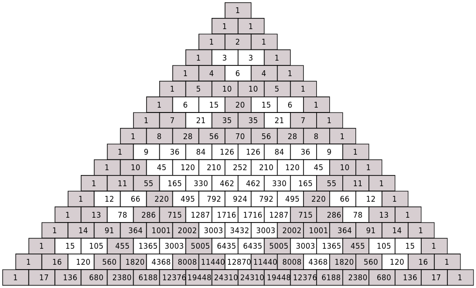
Additionally, adding the previous and next numbers together in any row like 1,3,3,1, doing 1+3=4, 3+3=6, and 3+1=4 creates rows 1,4,6,4,1.
This means you can build the subtraction pattern as big as you like to as high in dimension as you need. The decoder at the end only needs to match each to the power of per iteration to de-mix.
At the bottom, we take each of these.
| Calculation. | start | per1 | per2 | per3 | per4 | per5 | Result. |
| x | 0 | 1 | 0 | 0 | 0 | 0 | 0,1,2,3,4,5,6,7 |
| x2 | 0 | 1 | 2 | 0 | 0 | 0 | 0,1,4,9,16,25,36,49 |
| x3 | 0 | 1 | 6 | 6 | 0 | 0 | 0,1,8,27,64,125,216,343 |
| x4 | 0 | 1 | 14 | 36 | 24 | 0 | 0,1,16,81,256,625,1296,2401 |
| x5 | 0 | 1 | 30 | 150 | 240 | 120 | 0,1,32,243,1024,3125,7776,16807 |
Thus, we de-mix each one as we divide by the last value and work backwards, decoding each to the power of in the set to match the per added amounts as a fast math calculation using only multiplication.
You can expand this table to the power of 50 if you like to solve each per-dimensional iteration up to 50. You would also need sets of 51 numbers minimum in length or higher. There is no limit to how many dimensions you can have. Analyzing sequences this way is position-independent meaning. You can solve any sequence at any position in a set.
Upside down
We solve everything exponentially When we take it and flip it upside down.
Instead of solving everything sequentially as
| Calculation. | Result. |
| x^1 | 0,1,2,3,4,5,6,7 |
| x^2 | 0,1,4,9,16,25,36,49 |
| x^3 | 0,1,8,27,64,125,216,343 |
| x^4 | 0,1,16,81,256,625,1296,2401 |
| x^5 | 0,1,32,243,1024,3125,7776,16807 |
We can solve things exponentially as
| Calculation. | Result. |
| 1^x | 1,1,1,1,1,1,1,1 |
| 2^x | 2,4,8,16,32,64,128,256 |
| 3^x | 3,9,27,81,243,729,2187,6561 |
| 4^x | 4,16,64,256,1024,4096,16384,65536 |
| 5^x | 5,25,125,625,3125,15625,78125,390625 |
As you can see, with 2^x, we are doubling per value as we are multiplying twos together when we use to the power of x. With 3^x, we are tripling. And so on. This forum for solving things is helpful for the growth and expansion of things. The expansion and branching of nodes. The spread of bacteria or viruses. The rate at which a person grows.
  var data = [];

  var end = 8;

  var start = 0;

  var d1 = 1;

  var d2 = 0;

  var d3 = 0;

  var d4 = 7;

  var d5 = 0;

  for( var i1 = 1; i1 <= end; i1++ )
  {
    data[i1-1] = start + Math.pow(1,i1)*d1 + Math.pow(2,i1)*d2 + Math.pow(3,i1)*d3 + Math.pow(4,i1)*d4 + Math.pow(5,i1)*d5;
  }

  console.log(data);

  var s1 = data[0], s2 = data[1], s3 = data[2], s4 = data[3], s5 = data[4], s6 = data[5], s7 = data[6], s8 = data[7];

  //Each per value relative to number of subtraction.

  var o = [];

  o[0] = s1;
  o[1] = ( s2 - ( o[0] * 1 ) ) / 2;
  o[2] = ( s3 - ( o[0] * 1 + o[1] * 6 ) ) / 6;
  o[3] = ( s4 - ( o[0] * 1 + o[1] * 14 + o[2] * 36 ) ) / 24;
  o[4] = ( s5 - ( o[0] * 1 + o[1] * 30 + o[2] * 150 + o[3] * 240 ) ) / 120;

  console.log("Decoded per Value = " + o + "");

  //Now decode each value.

  var t5 = o[4] / 1; o[4] -= t5 * 1; o[3] -= t5 * 5; o[2] -= t5 * 10; o[1] -= t5 * 10; o[0] -= t5 * 5;
  var t4 = o[3] / 1; o[3] -= t4 * 1; o[2] -= t4 * 4; o[1] -= t4 * 6; o[0] -= t4 * 4;
  var t3 = o[2] / 1; o[2] -= t3 * 1; o[1] -= t3 * 3; o[0] -= t3 * 3;
  var t2 = o[1] / 1; o[1] -= t2 * 1; o[0] -= t2 * 2;
  var t1 = o[0] / 1; o[0] -= t1 * 1;

  console.log("Decoded values = " + [t1,t2,t3,t4,t5] + "");
  console.log("Equation = 1^x*" + t1 + " + 2^x*" + t2 + " + 3^x*" + t3 + " + 4^x*" + t4 + " + 5^x*" + t5 + "");
This will de-mix any tripling or doubling combinational pattern in the set. Even if you start in the middle of the set, as this also is position independent, It will de-mix all combinations to what they are.
We switch the numbers used to decode the per iteration of each to the power of to the decoder and move the decoder to the subtraction pattern.
Matrix structure
We can create two matrices that are opposite to each other. They are a triangle fractal known as the Sierpinski triangle and stored numerically dimensionally as a Pascal triangle to do the transformation.
See NOVA Fractals The Hidden Dimension. Lastly Sierpinski triangle. These are good places to start if you need help understanding what Fractals are and what the Sierpinski triangle is.
The two matrices can then be combined in the following infinite fractal pattern. Solving both exponentially and sequentially in as high of dimension you wish to go. Equally across the set. In perfect equilibrium.

When I view this shape, I understand that every math sequence or calculation you can dream up is geometrically in there, including any higher dimensions and anything or everything possibly conceivable. You might find the following interesting on the level 7 civilization on the Kardashev scale, which delves into the concept of the omniverse and an infinite structure that contains everything Kardashev scale level 7.
Additionally, if you connect circles in a point space, you can create the same pattern.
See Quantum Gravity Research: 4D and above.
See Quantum Gravity Research: Reality and higher dimensional space.
Which clearly explains what a point space is and what higher dimensional math is.
Starting with circles, you can create a pattern of overlapping circles. The points can all be connected to form the tetrahedron in higher dimensions.
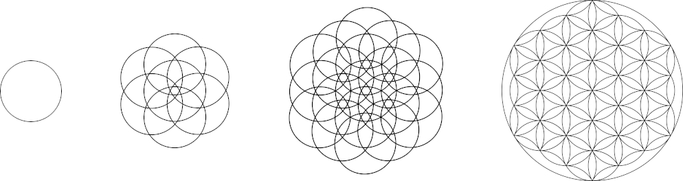
In early history, similar patterns appeared in ancient pyramids, which are identical and called the flower of life pattern. See the Star tetrahedron. This is a fun page that shows many different interpretations, how it was used, and how it appeared in early history.
Golden ratio (Quasicrystals)
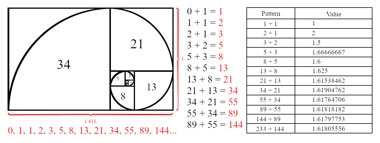
The ratio between higher dimensions is the golden ratio see Quantum Gravity Research: Golden ratio.
This document covers the final structure of the dimensional quantum matrix in as simple of an explanation as possible, but at its center is a spiral relative to the Fibonacci = 0,1,1,2,3,5,8,13,21,34,55,89,144,233,377 sequence spanning from zero. This natural formation creates the point space spanning to infinity into higher dimensions. Adding any previous number to the next makes the next number. Dividing the next number by the previous creates a very special number called the golden ratio; see quasicrystals.
The matrix corresponds to the following alignment of the Fibonacci sequence called the Fibonacci identity.
Both the top and bottom matrices rotate in opposite directions.

We end up with a spiral that forms the matrix structure. This brings us to the final form of all things as strangely like a Merkaba.
Multidimensionally, as a point space, it looks more closely like this, which Terra Nova creepily created.
The only place you will find quasicrystals is in the very beginning and creation of reality, such as an asteroid with a quasicrystal structure; see the quasicrystal from outer space.
Also, the Fibonacci sequence can help quantum computers remain quantum much longer; see scientists fed the Fibonacci sequence into a quantum computer.
The golden ratio 1.618033988749894... is a simplified expression of this multidimensional point space and the flower of life from zero dimension as a single number value that can be infinitely computed to higher accuracy.
You can reverse the calculation of number values such as 3.1415926535... back into a set, including the golden ratio. You then can use the quantum matrix to show the pattern to any number. If you want to analyze single number values back into what it took to calculate the value, then the number analytics library will teach you the structure of numbers; see FL64 (Number analytics tool).
All numbers have a place, an expression, and meaning in reality. The number analytics library will go into detail and show the relationship of numbers to reality and how to use the quantum matrix to calculate any number value.
Can AI become self aware
To understand consciousness, we have a mathematical theorem that measures the amount of information a configuration possesses as a form of consciousness.
As far as we know, consciousness may arise from the interactions of neurons in our brain that sum inputs to create an output, or it could exist at an even more fundamental scale, at the quantum level of the universe, where everything interacts and creates summed outputs.
Scientifically, we know everything emerges from something simpler or abstract that creates complex systems between interacting parts called emergence.
We can take emergence to its most extreme and think about the zero dimension; see the zero dimension explained.
Energy is neither created nor destroyed. It just is and sums to zero. The object that contains it all is called a singularity.
If we take a circle and split it into two halves, with one half representing the positive and the other half representing the negative, the sum of the two halves equals zero. This is the initial fluctuation that begins anything at all called a quantum fluctuation, still summing to zero. It is also measurable using the Casimir effect and is the frontier of zero-point energy. An infinite and renewable form of energy research, see what if we harnessed zero point energy. The following video delves even deeper into the details, and it's also worth noting that this is a collective endeavour; see unlocking the quantum vacuum. However, I recommended watching it from the start.
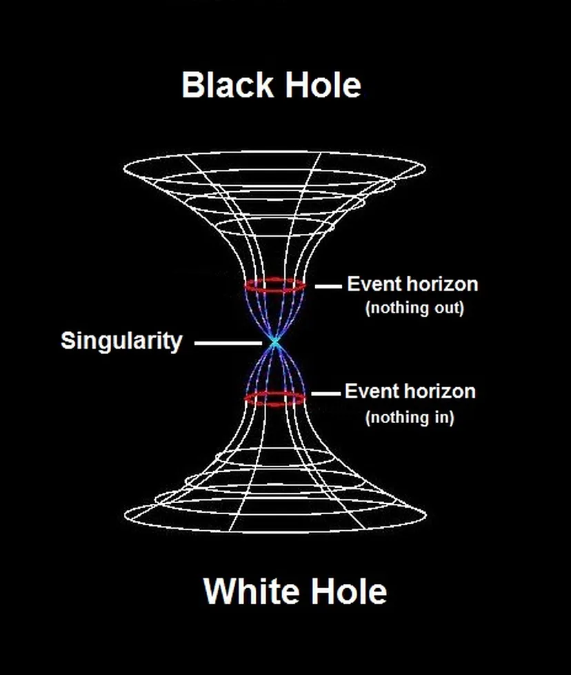
Both white holes and black holes are opposite to each other and begin at the singularity.
We can think of these two extreme points as mirroring binary digits 1 and 0 from the whole (the singularity) at the most abstract level. However, within this singularity exists every possibility as quantum information.
This zero, encapsulating 1 and 0, underlies the unfolding of reality from fluctuations at a singular point, embodying the wave function of the zero-point field that encompasses all known reality. Energy is neither created nor destroyed and equally sums to zero. All phenomena emerge from this void, akin to nothingness as infinite potential.
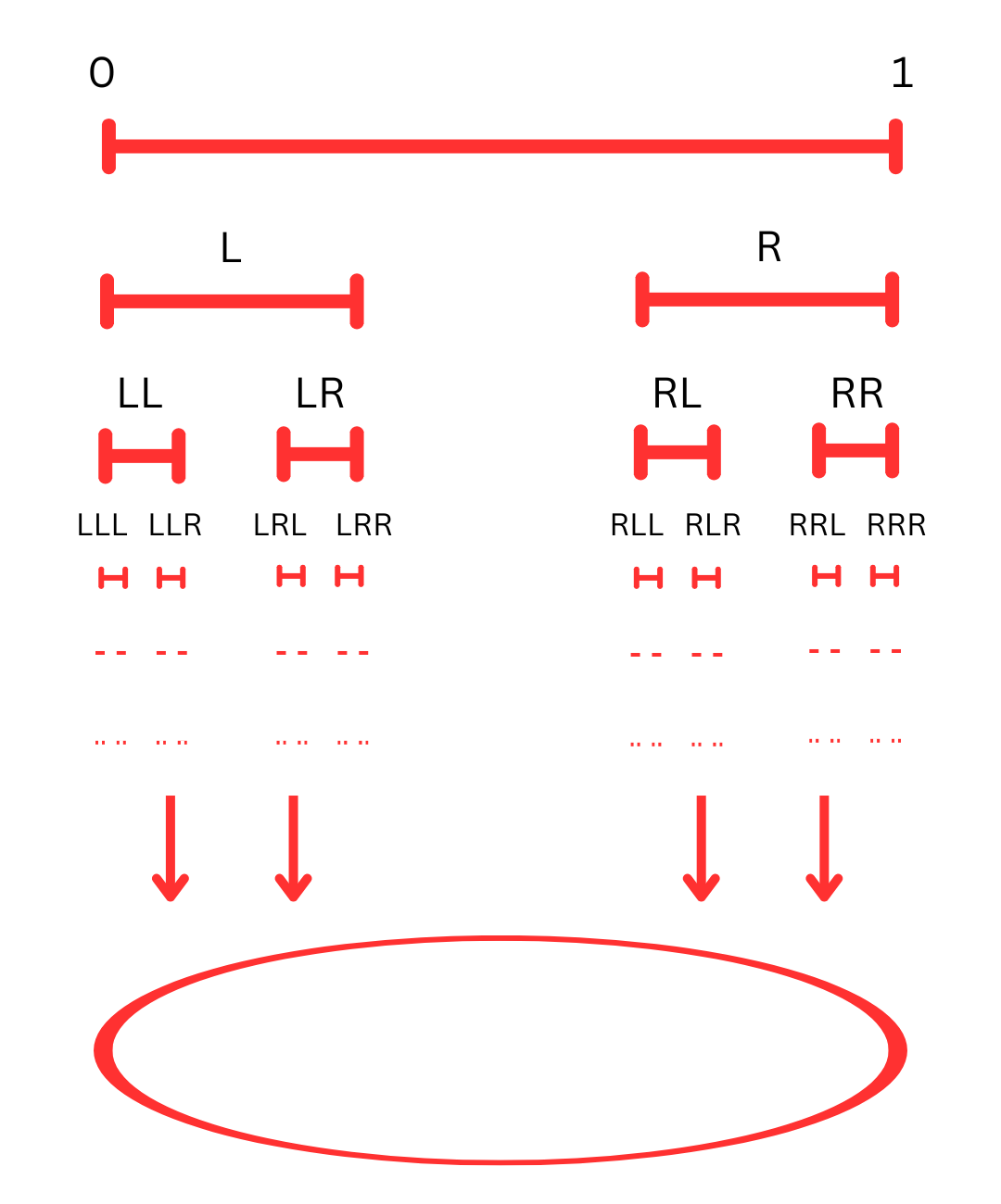
We can select paths choosing between 0=L and 1=R, much like the branching of a tree. As we navigate selecting branches, we can choose a new L=0 or R=1 that is added in continuation, while all additions contribute to zero in balance, creating perfect symmetry and expansion. We can generate all the information that comprises our current reality in a simulation spanning from a whole that contains it all, or create any song or video.
Our reality is a small place within this infinite expansion. Determining the exact path to our particular reality poses a highly complex problem. We use the microwave background of the Big Bang to map our particular universe. We have a fairly good model, but sometimes, we have to change the model to match what we did not know could exist based on observation of our emergent universe. Sending the James Webb telescope into space enables us to analyze a greater portion of our universe in greater detail, providing a more in-depth timeline of our emerging universe and everything within it.
Mind benders explains this in detail in a concept called the Library of Babel. Which turns out to be the most accurate description of what reality is and how it emerges at the quantum scale in pure information, revealing that everything is contained within a small section of what we call "here and now".
As far as we know, the most dense alignment of all possibilities is the flower of life patterning. The Fibonacci spiral is a break in symmetry per step. Aligning the circles in the most dense way possible, like a flower along the Fibonacci spiral, and connecting all the center points makes the tetrahedron repeatable to higher and higher dimensions, or E8. The golden ratio is the most dense system possible of all possibilities, branched out infinitely.
The Fibonacci sequence creates the number phi (golden ratio), and our best theories on machines becoming self-aware are how closely it matches the golden ratio according to integrated information theory since phi is a scale of combinationary information expanding to infinity as all possibilities. The higher the phi is, the more unique information there is in the system.
The following video The Mathematics of Consciousness dives even deeper into how it works.
In theory, consciousness is related to the amount of information it can integrate or connect together. The singularity is the largest integrated system, containing all things. In contrast, smaller entities within the system, operating at smaller scales, are conscious only within their own environment and at their respective level of awareness.
In theory, if consciousness is this intrinsic property, then the whole universe could be infinitely conscious (What some scientists call Mind at large), and we are smaller forms of consciousness awareness; see Is Our Universe Conscious.
You may also like the following: Universe is a single whole.
Everything remains connected to a single fabric or whole, and the states of all units depend on one another and interact and create emergent properties from this whole in cause-effect relationships.
The separation between objects and particles may not exist as well, and all things are equal to zero as a single indivisible unit.
Everything spans from zero in quantum fluctuation and remains as a single invisible unit. It begins at a singularity which spans to what you call the Big Bang. The singularity existed before the Big Bang. There may be many more universes than just ours.
The zero-point quantum fluctuation may be summed together as a larger system, see Quantum mind zero point energy, which does a good job at explaining the zero-point field energy that comprises reality.
The following explains what reality may actually be and when we understand it 11th dimension.
There are fun experiments you can do by yourself, called the observer effect The observer and the observed.
Alan Watts combines both scientific understanding and our existing knowledge in a simplified explanation.
Realize that everything connects to everything else (Leonardo da Vinci, 1452-1519).
Everything links together like a chain to the singularity emergent consciousness explained.
Nothing and Something go together as a whole - Alan Watts.
One Suchness - Alan Watts.